sum y
    Variable |        Obs        Mean    Std. dev.       Min        Max
-------------+---------------------------------------------------------
           y |        100    2.218156    2.082121   -2.61975   6.654652

EC3301 - Martinmas Semester
Consider a random sample (iid: independently and identitically distributed) drawn from the distribution
\[ y_i\sim N(2,25) \]
What is the \(\mu=E[y_i]\) and \(\sigma = \sqrt{Var(y_i)}\)?
Solve for the expected value and variance of the sample mean: \(\bar{y} = \frac{1}{n}\sum_{i=1}^n y_i\).
What is the distribution of \(\bar{y}\)?
Compute the probability that \(Pr(\bar{y}<3)\) in a sample of \(n=100\).
For the next few questions we will assume no knowledge of the true mean and variance of \(y\); only that the sample was drawn from a normal distribution \(y_i\sim N(\mu,\sigma^2)\). You draw a random sample of 100 observations from this distribution and the sample has the following characteristics:
sum y
Variable | Obs Mean Std. dev. Min Max
-------------+---------------------------------------------------------
y | 100 2.218156 2.082121 -2.61975 6.654652mean y
Mean estimation                            Number of obs = 100

--------------------------------------------------------------
             |       Mean   Std. err.     [95% conf. interval]
-------------+------------------------------------------------
           y |   2.218156   .2082121      1.805018    2.631294
--------------------------------------------------------------
What is the relationship between the standard deviation of the variable and the standard error of the sample mean reported above?
Earlier we showed that, \(\frac{\bar{y}-2}{sd(\bar{y})} \sim N(0,1)\) where \(sd(\bar{y}) = \sigma/\sqrt{n}\). Since we do not know \(\sigma\), what happens to the distribution if we replace \(\sigma\) with \(\hat{\sigma}\), the standard deviation of the sample.
Using the properties of the sample, test the null hypothesis \(H_0: \mu =1.85\). Use a significance level of \(\alpha = 0.05\).
Using the properties of the sample, test the null hypothesis \(H_0: \mu \leq 1.85\).
Why is the conclusion different for the two hypotheses?
Which test has more statistical power? Compute the power of the test to reject \(H_0\) when the true value of \(\mu = 2\).
In each case, try to prove the following properties of the OLS estimators (\(\hat{\beta_0},\hat{\beta_1}\)) for a simple linear regression model
\[ y_i = \beta_0 + \beta_1 x_i + u_i \]
\(\sum_{i=1}^n \hat{u}_i=0\), where \(\hat{u}_i = y_i - \hat{\beta}_0-\hat{\beta}_1 x_i\)
\(\bar{y} = \hat{\beta_0} + \hat{\beta_1} \bar{x}\), where \(\bar{y} = \frac{1}{n}\sum_{i=1}^n y_i\) and \(\bar{x} = \frac{1}{n}\sum_{i=1}^n x_i\).
\(\sum_{i=1}^n x_i \hat{u}_i = 0\)
\(\widehat{Cov}(x_i,\hat{u}_i)=0\) where \(\widehat{Cov}(\cdot,\cdot)\) is the sample covariance
One of the most widely estimated regression model in economics is the Mincer equation (Mincer 1974; Lemieux 2006). It is a simple linear regression model that regresses log of wages (or earnings) on years of education and a quadratic term in years of potential experience. Where potential experience is measured using years since school completion.
\[ \ln(wage_i) = \beta_0 + \beta_1 edu_i + \beta_2 exp_i + \beta_3 exp_i^2 + u_i \]
This simple model can be rationalized by a model in which workers choose the length of time the choose to remain in school and delay earning in income in the labour market (Card 2001).
Assuming \(E[u_i|edu_i,exp_i] = 0\), solve for \(\partial E[\ln(wage_i)|edu_i,exp_i]/\partial exp_i\). Is the \(E[\ln(wage_i)|edu_i,exp_i]\) concave or convex in years of experience?
Does it make sense to treat education as a continuous variable; i.e. years of education? What alternative approaches could you take?
For the remaing questions we are going to use a random sample of the 2024 CPS (Source: NBER MORG). The sample includes only male, full-time, workers and excludes self-employed workers. These estimates are based on a random sub-sample of 300 individuals from this dataset.
preserve
collapse (mean) wage, by(edu)
scatter wage edu, ytitle(Average wage) xtitle(Years of education)
restore
(Note: Below code run with echo to enable preserve/restore functionality.)
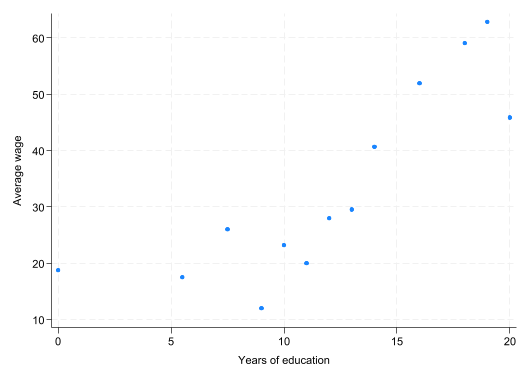
When working with micro-level data (i.e., unit is a firm, individual, household, etc.) you often need to aggregate the data to a lower level (e.g., region, group category). In Stata, this can be done using the collapse command. In R, you can use group_by() function within dplyr. This leads to an irreversible change in the structure of the dataset: you can aggregate data, but not disaggregate it. For this reason, it is a good idea to retain a version of the disaggregated data. In R, this is relatively straight forward because you can assign the aggregated file to a new dataframe. In Stata, you cannot have two datasets open at once. The solution therefore is to preserve a version of the disaggregated data and restore it once you are done with the aggregated file.
Note, preserve and restore must be run together. The command uses temporary files, so if you just run preserve and then later try to restore, the temporary file will no longer exist and you will need to re-open the disaggregated file and reproduce all other changes you made to the dataset.
preserve
collapse (mean) lnwage, by(edu)
scatter lnwage edu, ytitle(Average (log of) wage) xtitle(Years of education)
restore
(Note: Below code run with echo to enable preserve/restore functionality.)
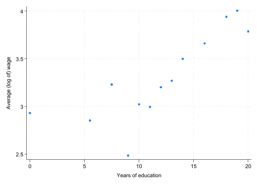
Below is an estimate of the Mincer equation using the same sub-sample:
reg lnwage edu exp expsq
      Source |       SS           df       MS      Number of obs   =       300
-------------+----------------------------------   F(3, 296)       =     33.82
       Model |  26.8176018         3  8.93920059   Prob > F        =    0.0000
    Residual |  78.2323313       296  .264298417   R-squared       =    0.2553
-------------+----------------------------------   Adj R-squared   =    0.2477
       Total |  105.049933       299  .351337569   Root MSE        =     .5141

------------------------------------------------------------------------------
      lnwage | Coefficient  Std. err.      t    P>|t|     [95% conf. interval]
-------------+----------------------------------------------------------------
         edu |   .0998468   .0107859     9.26   0.000       .07862    .1210736
         exp |   .0208725   .0081481     2.56   0.011      .004837    .0369081
       expsq |  -.0002387    .000162    -1.47   0.142    -.0005575    .0000801
       _cons |   1.732044   .1753344     9.88   0.000     1.386984    2.077104
------------------------------------------------------------------------------
Interpret the coefficient on edu.
Ask a LLM to provide an estimate of the returns to an additional year of education from the literature. You must specify that the outcome is measured in log-of wages. What is the typical estimate? And do our estimates seem off?
Can we reject the \(H_0: \beta_1 <0.08\) at a \(\alpha=0.01\) significance level? What if we chose \(\alpha=0.05\) instead?
Test the hypothesis that \(H_0:\beta_2=0\) at a \(\alpha=0.05\) significance level.
Test the hypothesis that \(H_0:\beta_3\geq0\) at a \(\alpha=0.05\) significance level.
Ignoring statistical significance, do the estimates suggest a concave or convex relationship with respect to years of experience?
If we take these estimates seriously, after how many years of experience do we expected wages to decline? Do wages decrease while workers are still working?
The following model was inspired by Frank and Goyal (2009) Capital Structure Decisions: Which Factors Are Reliably Important?. The authors use a database of publicly-traded (US-listed) firms, from 1950-2003. They have a rich dataset of firm-level and macro-economic variables. In this example, we do not have that. Instead, we have data from the most recent SEC filings for 2026-Q2. Using this smaller cross-sectional dataset, we can estimate the model:
\[ leverage_i = \beta_0 + \beta_1 size_i + \beta_2 profitability_i + \beta_3 tangibility_i + u_i \]
where,
leverage: total liabilities divided by total assetssize: log of total assetsprofitability: operating income divided by total assetstangibility: physical assets (e.g., property and equipment) divided by total assetsThe sample has been restricted to firms with assets of at least $1 million and a tangibility score within \([0,1]\).
sum leverage size profitability tangibility
    Variable |        Obs        Mean    Std. dev.       Min        Max
-------------+---------------------------------------------------------
    leverage |        271    1.311067    2.914094          0   22.16866
        size |        274     18.3593    2.601397   14.00696   26.29069
profitabil~y |        271    -.673556    2.286625  -29.20916   1.338037
 tangibility |        274    .1079863    .1624912          0   .9984815
reg leverage size profitability tangibility
      Source |       SS           df       MS      Number of obs   =       268
-------------+----------------------------------   F(3, 264)       =     29.28
       Model |    572.0114         3  190.670467   Prob > F        =    0.0000
    Residual |  1719.38448       264  6.51282001   R-squared       =    0.2496
-------------+----------------------------------   Adj R-squared   =    0.2411
       Total |  2291.39588       267  8.58200705   Root MSE        =     2.552

------------------------------------------------------------------------------
    leverage | Coefficient  Std. err.      t    P>|t|     [95% conf. interval]
-------------+----------------------------------------------------------------
        size |  -.2137509   .0642591    -3.33   0.001    -.3402764   -.0872253
profitabil~y |  -.5102825   .0724029    -7.05   0.000    -.6528431   -.3677218
 tangibility |    .868687   .9541517     0.91   0.363    -1.010029    2.747403
       _cons |   4.792315   1.208169     3.97   0.000     2.413441    7.171188
------------------------------------------------------------------------------
Interpret the \(\mathbf{R}^2\) measure. Is this a high or low value?
Interpret the _cons coefficient. Does this interpretation relate to a real firm?
Interpret each of the slope coefficients. For size, consider a 10% increase in assets. For profitability and tangibility, the regressor is a ratio. Consider the impact of an increase in the ratio of \(\Delta x = 0.01\) (or 1%).
These results are very different to those of Frank and Goyal (2009). For example, in their Table V the coefficient estimate for tangibility is \(0.092\). What are some of the factors that could explain our vastly different results.