Hypothesis Tests
Simple hypotheses
So far, we have considered hypotheses that involve a single estimator:
\(H_0: \beta_j=\kappa_0\)
\(H_0: \beta_j\geq \kappa_0\)
\(H_0: \beta_j\leq \kappa_0\)
Linear combinations
Today, we consider hypotheses of the form:
\[
H_0: a_0\beta_0 + a_1 \beta_1 + \cdots + a_k \beta_k = \kappa_0
\]
for constants \(\{a_j\}_{j=0,1,\dots,k}\) . This is a linear combination of parameters .
For example, \(H_0: \beta_1= 2\beta_2-0.5\) can be written as,
\[
H_0: \underbrace{0}_{a_0}\beta_0+\underbrace{1}_{a_1}\beta_1 +\underbrace{(- 2)}_{a_2}\beta_2 = \underbrace{-0.5}_{\kappa_0}
\]
Multiple linear combinations
Similarly, we could have \(q\) of these statements,
\[
\begin{aligned}
H_0: a^1_0\beta_0 + a^1_1 \beta_1 + \cdots + a^1_k \beta_k &= \kappa^1_0 \\
a^2_0\beta_0 + a^2_1 \beta_1 + \cdots + a^2_k \beta_k &= \kappa^2_0 \\
&\vdots \\
a^q_0\beta_0 + a^q_1 \beta_1 + \cdots + a^q_k \beta_k &= \kappa^q_0 \\
\end{aligned}
\]
Single linear combinations
Consider the following example related to environmental and health economics
\[
\ln(PM2.5_\ell) = \beta_0 + \beta_1 EV_\ell + \beta_2 hybrid_\ell + \mathbf{x}_\ell\gamma + u_\ell
\]
where,
\(PM2.5\) is micrograms of particulate matter (with diameter \(\leq 2.5\) micrometres) per cubic metre in location \(\ell\) .
standard measure for health effects as absorbable by lungs and bloodstream
\(EV\) and \(hybrid\) are number of registered vehicles (/1000) by fuel type in location \(\ell\) .
Example: PM2.5
The following estimates use local authority level data for 2019 in the UK.
Code
data "$data_dir\pm25.csv" , clear reg ln_pm25 ev_k hybrid_k petrol_k diesel_k ln_pop
(encoding automatically selected: ISO-8859-1)
(17 vars, 291 obs)

      Source |       SS           df       MS      Number of obs   =       291
-------------+----------------------------------   F(5, 285)       =     33.45
       Model |  2.84542086         5  .569084172   Prob > F        =    0.0000
    Residual |  4.84835963       285  .017011788   R-squared       =    0.3698
-------------+----------------------------------   Adj R-squared   =    0.3588
       Total |  7.69378049       290  .026530278   Root MSE        =    .13043

------------------------------------------------------------------------------
     ln_pm25 | Coefficient  Std. err.      t    P>|t|     [95% conf. interval]
-------------+----------------------------------------------------------------
        ev_k |   .0779783     .03734     2.09   0.038     .0044811    .1514755
    hybrid_k |   .0322276   .0063524     5.07   0.000      .019724    .0447312
    petrol_k |   .0000559   .0007053     0.08   0.937    -.0013323    .0014442
    diesel_k |   -.003546   .0005762    -6.15   0.000    -.0046802   -.0024119
      ln_pop |    .088135   .0208428     4.23   0.000     .0471096    .1291604
       _cons |   1.264753   .2325884     5.44   0.000     .8069436    1.722562
------------------------------------------------------------------------------
Code
# Load the Stata file <- read.csv (file.path (data_dir, "pm25.csv" ))# Estimate univariate linear regression <- lm (ln_pm25 ~ ev_k + hybrid_k + petrol_k + diesel_k + ln_pop, data = pm25_data)# View results summary (model1)
Call:
lm(formula = ln_pm25 ~ ev_k + hybrid_k + petrol_k + diesel_k +
    ln_pop, data = pm25_data)

Residuals:
     Min       1Q   Median       3Q      Max
-0.39959 -0.05714  0.03222  0.08413  0.47799

Coefficients:
              Estimate Std. Error t value Pr(>|t|)
(Intercept)  1.265e+00  2.326e-01   5.438 1.16e-07 ***
ev_k         7.798e-02  3.734e-02   2.088   0.0377 *
hybrid_k     3.223e-02  6.352e-03   5.073 7.06e-07 ***
petrol_k     5.591e-05  7.053e-04   0.079   0.9369
diesel_k    -3.546e-03  5.762e-04  -6.154 2.55e-09 ***
ln_pop       8.814e-02  2.084e-02   4.229 3.17e-05 ***
---
Signif. codes:  0 '***' 0.001 '**' 0.01 '*' 0.05 '.' 0.1 ' ' 1

Residual standard error: 0.1304 on 285 degrees of freedom
Multiple R-squared:  0.3698,    Adjusted R-squared:  0.3588
F-statistic: 33.45 on 5 and 285 DF,  p-value: < 2.2e-16
Null hypotheses
From a public policy perspective (if you consider designing subsidies), you want to estimate both \(\beta_1\) and \(\beta_2\) , BUT also know if
\[
H_0: \beta_1=\beta_2
\]
That is, should the policy discriminate bewteen electrified fuel types?
Engineers may be able provide mechanical differences, but they can’t tell you about differences in usage (driver behaviour) which is important for realized pollution mitigation.
Do not take these estimates too seriously. This model is a classic example of selection into “treatment”: those who live in higher pollution areas (e.g. dense urban centres) are also more likely to buy EVs. A better research design would use panel data to evaluate this question dyanmically.
Alternative hypothesis
The alternative in this case, may be
\[
H_1: \beta_1\neq \beta_2
\]
But may also be,
\[
H_1: \beta_1<\beta_2
\]
or
\[
H_1: \beta_1>\beta_2
\]
if there is a strong case for ruling out one case (see Wooldridge 2025, 139 ) .
Test statistic
For \(H_0: \beta_1=\beta_2\Rightarrow H_0:\beta_1-\beta_2=0\)
\[
\text{test-stat} = \frac{\hat{\beta}_1-\hat{\beta}_2}{\sqrt{Var(\hat{\beta}_1-\hat{\beta}_2)}}
\]
The more general case would be \(H_0: a_1\beta_1+a_2\beta_2=\kappa_0\)
\[
\text{test-stat} = \frac{a_1\hat{\beta}_1+a_2\hat{\beta}_2-\kappa_0}{\sqrt{Var(a_1\hat{\beta}_1+a_2\hat{\beta}_2)}}
\]
which can be extended to include more parameters.
Variance
The key to understanding and executing this test is,
\[
Var(\hat{\beta}_1-\hat{\beta}_2) \neq Var(\hat{\beta}_1) + Var(\hat{\beta}_2)
\]
This is because,
\[
\begin{aligned}
Var(a_1z_1+a_2z_2) =& Var(a_1z_1) + Var(a_2z_2) + 2\times Cov(a_1z_1,a_2z_2) \\
=&a_1^2Var(z_1) + a_2^2 Var(z_2) + 2\times a_1a_2Cov(z_1,z_2)
\end{aligned}
\]
for random variables \(z_1\) and \(z_2\) and constants \(a_1\) and \(a_2\) .
So,
\[
Var(\hat{\beta}_1-\hat{\beta}_2) = Var(\hat{\beta}_1) + Var(\hat{\beta}_2) - \textcolor{red}{2\times}\underbrace{\textcolor{blue}{Cov(\hat{\beta}_1,\hat{\beta}_2)}}_{\neq 0}
\]
Why \(-2\) ?
For this \(H_0\) ,
\[
\Rightarrow H_0: \underbrace{\beta_1-\beta_2 = 0}_{a_1\beta_1 + a_2\beta_2 = \kappa_0}
\]
So, \(a_1 = 1\) and \(a_2 = -1\) .
Distribution
Under MLR 1-6, the conditional distribution of this test-statistic is \(t_{n-k-1}\)
\[
t\text{-stat} = \frac{\hat{\beta}_1-\hat{\beta}_2}{\sqrt{Var(\hat{\beta}_1-\hat{\beta}_2)}}
\underset{H_0}{\sim} t_{n-k-1}
\]
under the null .
You can use the same steps from Lecture 3 to conduct inference: \(p\) -value, critical value.
We tend not to construct confidence intervals in such cases.
Similarly, you can compute the power under the alternative \(\beta_1-\beta_2 = \kappa\) .
Example: PM2.5
test lincom ev_k - hybrid_k
 ( 1)  ev_k - hybrid_k = 0

------------------------------------------------------------------------------
     ln_pm25 | Coefficient  Std. err.      t    P>|t|     [95% conf. interval]
-------------+----------------------------------------------------------------
         (1) |   .0457507   .0423487     1.08   0.281    -.0376053    .1291066
------------------------------------------------------------------------------
In R, you can use the marginaleffects package. However, this is NOT available in AppsAnywhere. Do not worry, there is an alternative coming up.
# Load package library (marginaleffects)# Estimate linear hypothesis hypotheses (model1, "ev_k - hybrid_k = 0" )
      Hypothesis Estimate Std. Error    z Pr(>|z|)   S   2.5 % 97.5 %
 ev_k-hybrid_k=0   0.0458     0.0423 1.08     0.28 1.8 -0.0373  0.129
Multiple linear hypotheses
Another common form of hypothesis concerns multiple linear combinations of estimators.
\[
\begin{aligned}
H_0: a^1_0\beta_0 + a^1_1 \beta_1 + \cdots + a^1_k \beta_k &= \kappa^1_0 \\
a^2_0\beta_0 + a^2_1 \beta_1 + \cdots + a^2_k \beta_k &= \kappa^2_0 \\
&\vdots \\
a^q_0\beta_0 + a^q_1 \beta_1 + \cdots + a^q_k \beta_k &= \kappa^q_0 \\
\end{aligned}
\]
You can think of this as a linear transformation of \(\beta\) .
\[
H_0: R\beta = r
\]
Where \(R\) is a \(q\times k\) matrix of constants and \(r\) a \(q\) -dimensional column vector of constants.
Example: PM2.5
In our example of
\[
PM2.5_\ell = \beta_0 + \beta_1 EV_\ell + \beta_2 hybrid_\ell + \mathbf{x}_\ell\gamma + u_\ell
\]
This could be as simple as,
\[
H_0: \beta_1 = 0\;\text{and}\; \beta_2 = 0
\]
Why not test \(H^{(1)}_0: \beta_1=0\) and then \(H^{(2)}_0: \beta_2 = 0\) as separate individual hypotheses? The combined size of these tests would not be \(\alpha\) . Why? The estimators are are correlated which implies:
\[
Pr\big(\text{Reject}\;H^{(1)}_0\;\text{or}\;H^{(2)}_0 \big|\beta_1=0,\beta_1=0\big) \neq \alpha
\]
There are a number of ways to correctly do multiple hypothesis testing. One is the Bonferroni correction which gets you to reject separate hypotheses sequentially using an algorithim. It does so by ensuring that the family-wise error rate (the probability of rejecting at least one true \(H_0\) across a “family” of hypotheses) is \(\leq \alpha\) .
Test
The test is performed by considering two models:
Unrestricted model; using our example,
\[
\ln(PM2.5_\ell) = \beta_0 + \beta_1 EV_\ell + \beta_2 hybrid_\ell + \mathbf{x}_\ell\gamma + u_\ell
\]
storing the \(SSR_{ur}\) from this model
Restricted model , which imposes \(H_0: \beta_1 = 0\;\text{and}\; \beta_2 = 0\) ,
\[
\ln(PM2.5_\ell) = \beta_0 + \mathbf{x}_\ell\gamma + u_\ell
\]
storing the \(SSR_{r}\) from this model
Test statistic
The test static that is then given by,
\[
F\text{-stat} = \frac{(SSR_{r}-SSR_{ur})/q}{SSR_{ur}/df_{ur}}
\]
where,
\(SSR_r\) and \(SSR_{ur}\) come from the restricted (\(r\) ) and unrestricted models (\(ur\) ).
\[
SSR_{r}-SSR_{ur}>0
\]
Test statistic
The test static that is then given by,
\[
F\text{-stat} = \frac{(SSR_{r}-SSR_{ur})/q}{SSR_{ur}/df_{ur}}
\]
and,
Distribution
Under the null, \(F\) -stat has an \(F\) distribution (hence the name)
\[
F\text{-stat} \underset{H_0}{\sim}F_{q,n-k-1}
\]
We reject \(H_0\) if
\[
F\text{-stat} > F_{q,n-k-1}^{-1}(1-\alpha) = f_{q,n-k-1,1-\alpha}
\]
where \(F_{q,n-k-1}^{-1}(1-\alpha)\) is the \(1-\alpha\) percentile of the distribution.
Rejection rule
\[
F\text{-stat} > f_{q,n-k-1,1-\alpha}
\]
Doesn’t mean that \(H_1\) is one-sided.
You cannot tell which direction the deviation from the null is, because F-stat uses squared-deviations (i.e. sign is lossed) .
\(H_1:\; H_0\;\text{false}\) , or \(H_1: \beta_1\neq0\;\text{or}\; \beta_2\neq0\)
The \(F\) distribution is defined as the ratio of two chi-squared distributions,
\[
F_{q,m} = \frac{\chi^2_q/q}{\chi^2_m/m}
\]
each normalized by their corresponding degrees of freedom.
Example: PM2.5
F -test test ev_k hybrid_k
 ( 1)  ev_k = 0
 ( 2)  hybrid_k = 0

       F(  2,   285) =   53.88
            Prob > F =    0.0000
In R, you can use the car package, which is available in AppsAnywhere.
# Load package library (car)# Estimate linear hypothesis linearHypothesis (model1, c ("ev_k = 0" , "hybrid_k = 0" ))
Linear hypothesis test:
ev_k = 0
hybrid_k = 0

Model 1: restricted model
Model 2: ln_pm25 ~ ev_k + hybrid_k + petrol_k + diesel_k + ln_pop

  Res.Df    RSS Df Sum of Sq      F    Pr(>F)
1    287 6.6816
2    285 4.8484  2    1.8332 53.881 < 2.2e-16 ***
---
Signif. codes:  0 '***' 0.001 '**' 0.01 '*' 0.05 '.' 0.1 ' ' 1
Revisiting single linear restriction
You can think of a single linear hypothesis as a special case of multiple where \(q=1\) . For example,
\[
H_0: \textcolor{red}{\beta_1} = \textcolor{blue}{\beta_2}
\]
Restricted model:
\[
\begin{aligned}
\ln(PM2.5_\ell) =& \beta_0 + \textcolor{red}{\beta_1} EV_\ell + \underbrace{\textcolor{red}{\beta_1}}_{=\textcolor{blue}{\beta_2}} hybrid_\ell + \mathbf{x}_\ell\gamma + u_\ell \\
= & \beta_0 + \textcolor{red}{\beta_1} (EV_\ell + hybrid_\ell) + \mathbf{x}_\ell\gamma + u_\ell
\end{aligned}
\]
A regression with a new transformed variable: \(EV_\ell + hybrid_\ell\)
Moreover, you can show that for \(q=1\)
\[
F\text{-stat} = \frac{SSR_{r}-SSR_{ur}}{SSR_{ur}/(n-k-1)} = (t\text{-stat})^2
\]
Example: PM2.5
Code
test lincom ev_k - hybrid_kF -test test ev_k=hybrid_ksqrt (r (F ))
 ( 1)  ev_k - hybrid_k = 0

------------------------------------------------------------------------------
     ln_pm25 | Coefficient  Std. err.      t    P>|t|     [95% conf. interval]
-------------+----------------------------------------------------------------
         (1) |   .0457507   .0423487     1.08   0.281    -.0376053    .1291066
------------------------------------------------------------------------------


 ( 1)  ev_k - hybrid_k = 0

       F(  1,   285) =    1.17
            Prob > F =    0.2809

1.0803322
Code
# t-test hypotheses (model1, "ev_k - hybrid_k = 0" )
      Hypothesis Estimate Std. Error    z Pr(>|z|)   S   2.5 % 97.5 %
 ev_k-hybrid_k=0   0.0458     0.0423 1.08     0.28 1.8 -0.0373  0.129
Code
# F-test linearHypothesis (model1, "ev_k = hybrid_k" )
Linear hypothesis test:
ev_k - hybrid_k = 0

Model 1: restricted model
Model 2: ln_pm25 ~ ev_k + hybrid_k + petrol_k + diesel_k + ln_pop

  Res.Df    RSS Df Sum of Sq      F Pr(>F)
1    286 4.8682
2    285 4.8484  1  0.019855 1.1671 0.2809
Regression significance
A special case of this form of test concerns the joint significance of all the slope parameters in a model:
\[
H_0: \beta_1 = 0,\; \beta_2 = 0,\;\dots,\;\beta_k=0
\]
In this case,
The restricted model is a regression on a constant (alone) where \(\Rightarrow \mathbf{R}^2_{r}=0\)
And \(\mathbf{R}^2_{ur}\) is simply the \(\mathbf{R}^2\) from the model
The number of restrictions is \(q=k\)
We define the \(F\) -stat as,
\[
F\text{-stat} = \frac{\mathbf{R}^2/k}{(1-\mathbf{R}^2)/(n-k-1)}
\]
Structural Change
Dummy variables: recap
Recall, when we have the model:
\[
y_i = \beta_0 + \beta_1 d_i + u_i
\]
where \(d_i\in\{0,1\}\) . Then,
\[
\beta_1 = E[y_i|d_i=1]-E[y_i|d_i=0]
\]
Dummy variable interactions
Now, suppose the model was
\[
y_i = \beta_0 + \beta_1 x_i + \beta_2 d_i + \beta_3 x_i\times d_i + u_i
\]
where \(x_i\) is continuous.
What is the interpretation of each parameter?
\[
y_i = \beta_0 + \beta_1 x_i + \beta_2 d_i + \beta_3 x_i\times d_i + u_i
\]
\(\beta_0=E[y_i|\textcolor{blue}{d_i=0},x_i=0]\)
\(\beta_1 = \frac{dE[y_i |\textcolor{blue}{d_i=0},x_i]}{dx_i}\)
\(\beta_2=E[y_i|\textcolor{red}{d_i=1},x_i=0]-E[y_i|\textcolor{blue}{d_i=0},x_i=0]\)
\(\beta_3 = \frac{dE[y_i |\textcolor{red}{d_i=1},x_i]}{dx_i}-\frac{dE[y_i |\textcolor{blue}{d_i=0},x_i]}{dx_i}\)
Another way of thinking about it:
For \(d_i=0\) , the model is:
\[
y_i = \textcolor{blue}{\beta_0} + \textcolor{blue}{\beta_1} x_i + u_i
\]
For \(d_i = 1\) , the model is:
\[
y_i = \beta_0 + \beta_1 x_i + \beta_2 + \beta_3 x_i + u_i
\]
Which can be rewritten as:
\[
y_i = \underbrace{(\beta_0 + \beta_2)}_{\textcolor{red}{\gamma_0}} + \underbrace{(\beta_1 + \beta_3)}_{\textcolor{red}{\gamma_1}} x_i + u_i
\]
We have two models: for \(d_i=0\) and \(d_i=1\) .
Example
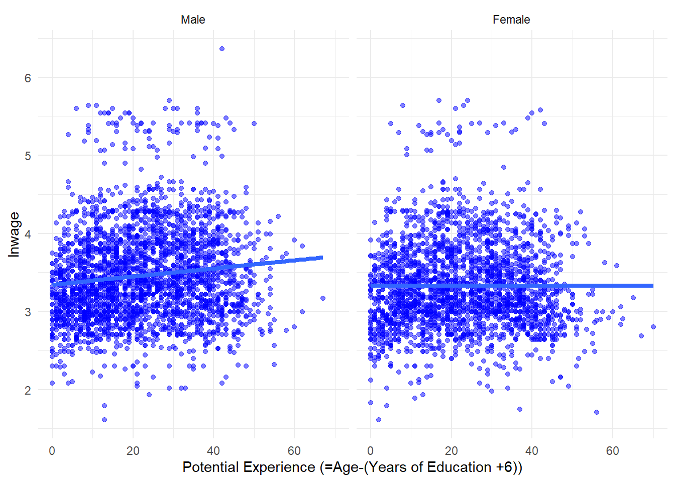
The typical example is the returns to education for men and women (as in Wooldridge 2025, 243 )
But, given what we know about the ‘parent penalty’ (Kleven et al. 2019 ) , it seems more pertinent to focus on experience
\[
\ln(wage_i) = \beta_0 + \beta_1 exp_i + u_i
\]
Code
use "$data_dir\morg24_bothgen.dta" , clear twoway (scatter lnwage exp , mc(blue %50)) (lfit lnwage exp , lwidth(*2)), by (sex, legend (off ) note ("" ) ) xtitle ("Potential Experience (=Age-(Years of Education +6))" )
Code
<- read_dta (file.path (data_dir, "morg24_bothgen.dta" ))ggplot (wage_data, aes (x = exp, y = lnwage)) + geom_point (colour = "blue" , alpha = 0.5 ) + geom_smooth (method = "lm" , se = FALSE , linewidth = 1.5 ) + facet_wrap (~ as_factor (sex)) + labs (x = "Potential Experience (=Age-(Years of Education +6))" ) + theme_minimal ()
`geom_smooth()` using formula = 'y ~ x'
If we overlay the fitted lines we get
Code
fitted linestwoway (lfit lnwage exp if sex==1, lc(blue )) (lfit lnwage exp if sex==2, lc(red ) lwidth(*2)), xtitle ("Potential Experience (=Age-(Years of Education +6))" ) legend (order (1 "Male" 2 "Female" ) r (2) ring (0) pos(5)) ylabel (2(1)6)
Code
$ group <- factor (wage_data$ sex, levels = c (1 , 2 ),labels = c ("Male" , "Female" ))ggplot (wage_data, aes (x = exp, y = lnwage, colour = group)) + geom_smooth (data = subset (wage_data, sex == 1 ),method = "lm" , se = FALSE , linewidth = 0.75 ) + geom_smooth (data = subset (wage_data, sex == 2 ),method = "lm" , se = FALSE , linewidth = 1.5 ) + scale_colour_manual (values = c (Male = "blue" , Female = "red" )) + scale_y_continuous (breaks = 2 : 6 ) + coord_cartesian (ylim = c (2 , 6 )) + labs (x = "Potential Experience (=Age-(Years of Education +6))" ,y = "lnwage" , colour = NULL ) + theme_minimal () + / theme (legend.position = "inside" ,legend.position.inside = c (0.98 , 0.02 ),legend.justification = c (1 , 0 ))
Error in parse(text = input): <text>:14:20: unexpected '/'
13:        y = "lnwage", colour = NULL) +
14:   theme_minimal() +/
                       ^
\(F\) -testThe \(F\) -test can be used to test differences in a model across groups.
For example, whether the Mincer equation (from Tutorial 1 ) differs by gender.
\[
\ln(wage_i) = \beta_0 + \beta_1 edu_i + \beta_2 exp_i + u_i
\]
We estimated this model for the male-only sample
The quadratic term in \(exp\) has been dropped for simplification
The model has \(k+1=3\) parameters
Test:
We may wish to ask whether:
is the same as,
Null hypothesis
This question implies a null hypothesis:
\[
H_0: \textcolor{blue}{\beta_0} = \textcolor{red}{\gamma_0},\;\textcolor{blue}{\beta_1} = \textcolor{red}{\gamma_1},\;\textcolor{blue}{\beta_2} = \textcolor{red}{\gamma_2}
\]
against,
\[
H_1: H_0\;\text{false}
\]
Approach 1
The \(F\) -test for this hypothesis has the form:
\[
F\text{-stat} = \frac{(SSR_P - (\textcolor{blue}{SSR_1} + \textcolor{red}{SSR_2}))/(k+1)}{(\textcolor{blue}{SSR_1} + \textcolor{red}{SSR_2})/(n-2(k+1))}
\]
where,
\(SSR_P\) is the “pooled” (\(P\) ) \(SSR\) from a regression of the joint sample.
\(\textcolor{blue}{SSR_1}\) is the \(SSR\) from a regression for just group 1.
\(\textcolor{red}{SSR_2}\) is the \(SSR\) from a regression for just group 2.
together \(\textcolor{blue}{SSR_1}\) and \(\textcolor{red}{SSR_2}\) represent the unrestricted model.
\(n-2(k+1)\) is the combined degrees of freedom from group 1 and 2.
\(k+1\) parameters are estimated in each group.
Distribution
The \(F\) -stat is (unsurprisingly) \(F\) -distributed,
\[
F\text{-stat} \underset{H_0}{\sim} F_{k+1,n-2(k+1)}
\]
Approach 2
This test has an equivalent form using interactions. Let,
\[
d_i= \mathbf{1}\{\text{`Group 2'}\}
\]
For example,
\[
d_i= \mathbf{1}\{\text{`Female'}\}
\]
Interactions
We can write the unrestricted model as,
\[
\ln(wage_i) = \beta_0 + \beta_1 edu_i+\beta_2 exp_i +\beta_3 d_i + \beta_4 edu_i\times d_i + \beta_5 exp_i\times d_i +u_i
\]
We now have 6 parameters: \(2\times (k+1)\) (for \(k=2\) )
As before, the dummy and dummy-interactions tell you about differences,
\[
\beta_3 = E[\ln(wage_i)|\textcolor{red}{d_i=1},edu_i=0,exp_i=0]-E[\ln(wage_i)|\textcolor{blue}{d_i=0},edu_i=0,exp_i=0]
\]
and
\[
\beta_j = \frac{\partial E[\ln(wage_i)|\textcolor{red}{d_i=1},edu_i,exp_i]}{\partial x_{ij}}-\frac{\partial E[\ln(wage_i)|\textcolor{blue}{d_i=0},edu_i,exp_i]}{\partial x_{ij}} \qquad j=4,5
\]
Test
Intuitively, the test for whether the model differs by group is given by,
\[
H_0: \beta_3 = 0,\;\beta_4=0,\;\beta_5=0
\]
where,
unrestricted model is given by,
\[
\ln(wage_i) = \beta_0 + \beta_1 edu_i+\beta_2 exp_i +\beta_3 d_i + \beta_4 edu_i\times d_i + \beta_5 exp_i\times d_i +u_i
\]
restricted model is given by,
\[
\ln(wage_i) = \beta_0 + \beta_1 edu_i + \beta_2 exp_i +v_i
\]
\(F\) -statThe \(F\) -stat is given by,
\[
F\text{-stat} = \frac{(SSR_{r}-SSR_{ur})/3}{SSR_{ur}/(n-6)}
\]
Compare this to the first approach:
\[
F\text{-stat} = \frac{(SSR_P - (\textcolor{blue}{SSR_1} + \textcolor{red}{SSR_2}))/3}{(\textcolor{blue}{SSR_1} + \textcolor{red}{SSR_2})/(n-6)}
\]
Equivalence
These two test-statics are equivalent because,
\(SSR_P=SSR_r\)
\(\textcolor{blue}{SSR_1} +\textcolor{red}{SSR_2} = SSR_{ur}\)