Tutorial 1 (Solutions)

EC3301 - Martinmas Semester

Statistical inference

Consider a random sample (iid: independently and identitically distributed) drawn from the distribution

\[ y_i\sim N(2,25) \]

What is the $\mu=E[y_i]$ and $\sigma = \sqrt{Var(y_i)}$?

\[ \begin{aligned} \mu = 2 \\ \sigma = 5 \end{aligned} \]

Solve for the expected value and variance of the sample mean: $\bar{y} = \frac{1}{n}\sum_{i=1}^n y_i$.

\[ \begin{aligned} E[\bar{y}] =& E\Bigg[\frac{1}{n}\sum_{i=1}^n y_i\Bigg] \\ =& \frac{1}{n}\sum_{i=1}^n E[y_i] \\ =& \frac{1}{n}\sum_{i=1}^n 2 \\ =& \frac{2n}{n} \\ =& 2 \end{aligned} \]

\[ \begin{aligned} Var(\bar{y}) =& E[(\bar{y}-\underbrace{E[\bar{y}]}_{=2})^2] \\ =& E\Bigg[\bigg(\frac{1}{n}\sum_{i=1}^n (y_i-2)\bigg)^2\Bigg] \\ =& E\Bigg[\frac{1}{n^2}\sum_{i=1}^n (y_i-2)^2+2\times\frac{1}{n^2}\sum_{i=1}^{n-1} \sum_{j=i+1}^{n} (y_i-2)(y_j-2)\Bigg] \\ =& \frac{1}{n^2}\sum_{i=1}^n \underbrace{E\big[(y_i-2)^2\big]}_{Var(y_i)} + 2\times \sum_{i=1}^{n-1} \sum_{j=i+1}^{n} \underbrace{E\big[(y_i-2)(y_j-2)\big]}_{Cov(y_i,y_j)=0} \\ =& \frac{nVar(y_i)}{n^2} \\ =& \frac{25}{n} \end{aligned} \]

What is the distribution of $\bar{y}$?

\[ \bar{y} \sim N(2,25/n) \]

Compute the probability that $Pr(\bar{y}<3)$ in a sample of $n=100$.

Since $\bar{y} \sim N(2,1/4)$,

\[ \frac{\bar{y}-2}{0.5} \sim N(0,1) \]

\[ \begin{aligned} Pr(\bar{y}<3) =& Pr(\bar{y}-2<3-2) \\ =& Pr\bigg(\frac{\bar{y}-2}{0.5} < \frac{1}{0.5}\bigg) \\ =& Pr(z<2) \end{aligned} \]

dis normal(2)

.97724987

For the next few questions we will assume no knowledge of the true mean and variance of $y$; only that the sample was drawn from a normal distribution $y_i\sim N(\mu,\sigma^2)$. You draw a random sample of 100 observations from this distribution and the sample has the following characteristics:

sum y


    Variable |        Obs        Mean    Std. dev.       Min        Max
-------------+---------------------------------------------------------
           y |        100    2.218156    2.082121   -2.61975   6.654652

mean y


Mean estimation                            Number of obs = 100

--------------------------------------------------------------
             |       Mean   Std. err.     [95% conf. interval]
-------------+------------------------------------------------
           y |   2.218156   .2082121      1.805018    2.631294
--------------------------------------------------------------

What is the relationship between the standard deviation of the variable and the standard error of the sample mean reported above?

The reported standard deviation is the square-root of the sample variance. The sample variance ($\hat{\sigma}^2$) is an estimate of the unobserved distribution variance ($\sigma^2$). In this sample, $\hat{\sigma} = 2.082121$. Note, the estimator is

\[ \hat{\sigma}^2 = \frac{1}{n-1}\sum_{i=1}^n (y_i-\bar{y})^2 \]

where division by $n-1$ results from the fact that the demeaned $y$ has $n-1$ degrees of freedom (since the variable has mean zero). It is for this same reason that the $t$-distribution in Q.6 has $n-1$ degrees of freedom.

The reported standard error is the square root of the $Var(\bar{y})$. As we proved above, $Var(\bar{y}) = \sigma^2/n$. That means that $sd(\bar{y}) = \sigma/\sqrt{n}$.

However, we do not know the true value of $\sigma$. In our estimation of the $sd(\bar{y})$, we replace $\sigma$ with $\hat{\sigma}$: $se(\bar{y}) = \hat{\sigma}/\sqrt{n}$.

As $n=100$, we find that $se = 0.2082121$; exactly equal to the $\hat{\sigma}/10$.

Earlier we showed that, $\frac{\bar{y}-2}{sd(\bar{y})} \sim N(0,1)$ where $sd(\bar{y}) = \sigma/\sqrt{n}$. Since we do not know $\sigma$, what happens to the distribution if we replace $\sigma$ with $\hat{\sigma}$, the standard deviation of the sample.

\[ \frac{\bar{y}-2}{\hat{\sigma}/\sqrt{n}} \sim t_{n-1} \]

Using the properties of the sample, test the null hypothesis $H_0: \mu =1.85$. Use a significance level of $\alpha = 0.05$.

\[ \frac{\bar{y}-1.85}{\hat{\sigma}/\sqrt{n}} \underset{H_0}{\sim} t_{n-1} \]

Compute the test statistic:

dis (_b[y]-1.85)/_se[y]

1.7681755

Using stored estimates

The mean command stores estimates in a similar way to regress. They are both e-class commands.

The _b[] function can be used to call the stored coefficient estimate for a particular variable. The full set of coefficients is stored as in the vector e(b).
The _se[] function can be used to call the SE of a particular coefficient. This is computed using the covariance matrix stored as e(V).

To see the full list of stored estimates, type ereturn list. Note, this does not work for summarize, which is a r-class command. After sum you can run return list to see the format of its stored estimates.

It is good practice to used stored estimates in this way as it prevents typing errors and improves replicability.

R users tend define a model as a list before summarizing it: e.g. model <- lm(yvar ~ xvar, data) followed by summary(model). You can then reference the slope coefficient of the stored model using coef(model)["xvar"] or model$coefficients["xvar"] (replacing xvar with the name of the variable). The get the standard error, you need to do a bit more work: summary(model)$coefficients["xvar", "Std. Error"] references a value from the summary or sqrt(diag(vcov(model)))["xvar"] (compute the square-root of the diagonal of the covariance matrix).

Rejection rule:

Since this is a two-sided test, we will reject if $|t\text{-stat}|<\text{t}_{99,0.975}$.

The test static remains the same.

Critical values of $t$-distribution (which is symmetric):

dis invt(99,0.975)

1.984217

Since $|t\text{-stat}|<\text{t}_{99,0.975}$, we fail to reject.

Using the properties of the sample, test the null hypothesis $H_0: \mu \leq 1.85$.

Rejection rule:

Since this is a one-sided test, we will reject if $t\text{-stat}>\text{t}_{99,0.95}$.

Critical values of $t$-distribution (which is symmetric):

dis invt(99,0.95)

1.6603912

We reject $H_0$ and conclude that $\mu > 1.85$.

Why is the conclusion different for the two hypotheses?

The only difference is the critical value. The one-side test has a lower critical value than the two-sided test.

Which test has more statistical power? Compute the power of the test to reject $H_0$ when the true value of $\mu = 2$.

In the two-sided test:

\[ \begin{aligned} Pr(\text{Reject}\;H_0|\mu = 2) =& Pr\Bigg(\bigg|\frac{\bar{y}-1.85}{se}\bigg|>\text{t}_{99,0.975}\Bigg|\mu = 2\Bigg) \\ =& Pr\Bigg(\frac{\bar{y}-1.85}{se}<\text{t}_{99,0.025}\Bigg|\mu = 2\Bigg) + Pr\Bigg(\frac{\bar{y}-1.85}{se}>\text{t}_{99,0.975}\Bigg|\mu = 2\Bigg) \\ =& Pr\Bigg(\frac{\bar{y}-2}{se}<\text{t}_{99,0.025}-\frac{0.15}{se}\Bigg|\mu = 2\Bigg) \\ &+ Pr\Bigg(\frac{\bar{y}-2}{se}>\text{t}_{99,0.975}-\frac{0.15}{se}\Bigg|\mu = 2\Bigg) \\ =& t_{n-1}\big(\text{t}_{99,0.025}-0.15/se\big) + 1-t_{n-1}\big(\text{t}_{99,0.975}-0.15/se\big) \\ \end{aligned} \]

where $t_{n-1}(\cdot)$ is the CDF of the $t$-distribution.

dis t(99,invt(99,0.025)-0.15/_se[y]) + 1 - t(99,invt(99,0.975)-0.15/_se[y])

.10866073

In the one-sided test:

\[ \begin{aligned} Pr(\text{Reject}\;H_0|\mu = 2) =& Pr\Bigg(\frac{\bar{y}-1.85}{se}>\text{t}_{99,0.95}\Bigg|\mu = 2\Bigg) \\ =& Pr\Bigg(\frac{\bar{y}-2}{se}>\text{t}_{99,0.95}-\frac{0.15}{se}\Bigg|\mu = 2\Bigg) \\ =& 1-t_{n-1}\big(\text{t}_{99,0.95}-0.15/se\big) \\ \end{aligned} \]

dis 1 - t(99,invt(99,0.95)-0.15/_se[y])

.17475989

This shows that the one-sided test is a more powerful test.

The OLS estimator

In each case, try to prove the following properties of the OLS estimators ($\hat{\beta_0},\hat{\beta_1}$) for a simple linear regression model

\[ y_i = \beta_0 + \beta_1 x_i + u_i \]

$\sum_{i=1}^n \hat{u}_i=0$, where $\hat{u}_i = y_i - \hat{\beta}_0-\hat{\beta}_1 x_i$

Substitute in the definitions of $\hat{\beta}_0$:

\[ \begin{aligned} \sum_{i=1}^n \hat{u}_i =& \sum_{i=1}^n \big(y_i - (\bar{y}-\hat{\beta}_1\bar{x})-\hat{\beta}_1 x_i\big) \\ =& \sum_{i=1}^n\big( (y_i - \bar{y})-\hat{\beta}_1 (x_i-\bar{x})\big) \\ =& \underbrace{\sum_{i=1}^n (y_i - \bar{y})}_{=0} + \hat{\beta}_1 \underbrace{\sum_{i=1}^n(x_i-\bar{x})}_{=0} \\ =& 0 \end{aligned} \]

This demonstrates that the intercept plays an important role in ensuring this result.

$\bar{y} = \hat{\beta_0} + \hat{\beta_1} \bar{x}$, where $\bar{y} = \frac{1}{n}\sum_{i=1}^n y_i$ and $\bar{x} = \frac{1}{n}\sum_{i=1}^n x_i$.

This follows from the definition of $\hat{\beta_0}$, but can also be shown using the decomposition of $y_i = \hat{y}_i + \hat{u}_i$

\[ \begin{aligned} \frac{1}{n}\sum_{i=1}^n y_i =& \frac{1}{n}\sum_{i=1}^n \hat{y}_i + \underbrace{\frac{1}{n}\sum_{i=1}^n\hat{u}_i}_{=0} \\ =& \frac{1}{n}\sum_{i=1}^n (\hat{\beta_0} + \hat{\beta_1}x_i) \\ =& \hat{\beta_0} + \hat{\beta_1}\frac{1}{n}\underbrace{\sum_{i=1}^n x_i}_{\bar{x}} \end{aligned} \]

$\sum_{i=1}^n x_i \hat{u}_i = 0$

Substitute in the definitions of $\hat{u}_i$ from 1.

\[ \sum_{i=1}^n x_i \hat{u}_i =\sum_{i=1}^n x_i (y_i - \hat{\beta}_0-\hat{\beta}_1 x_i) \]

Now substitue in $\hat{\beta}_0$ and re-arrange

\[ = \sum_{i=1}^n x_i (y_i - \bar{y}) -\hat{\beta}_1 \sum_{i=1}^nx_i(x_i-\bar{x}) \]

Substitute in the definition of $\hat{\beta}_1$

\[ \begin{aligned} =& \sum_{i=1}^n x_i (y_i - \bar{y}) -\frac{\sum_{i=1}^n (x_i-\bar{x})(y_i-\bar{y})}{\sum_{i=1}^n(x_i-\bar{x})^2} \sum_{i=1}^nx_i(x_i-\bar{x}) \\ =& 0 \end{aligned} \]

The result follows from the fact that,

\[ \sum_{i=1}^n x_i (y_i - \bar{y}) = \sum_{i=1}^n (x_i-\bar{x})(y_i-\bar{y}) \] and,

\[ \sum_{i=1}^nx_i(x_i-\bar{x}) = \sum_{i=1}^n(x_i-\bar{x})(x_i-\bar{x})=\sum_{i=1}^n(x_i-\bar{x})^2 \]

See Lecture 2 and Wooldridge pp. 27 and pp. 757.

$\widehat{Cov}(x_i,\hat{u}_i)=0$ where $\widehat{Cov}(\cdot,\cdot)$ is the sample covariance

The result follows directly from 1. and 3.

\[ \begin{aligned} \widehat{Cov}(x_i,\hat{u}_i) =& \frac{1}{n-1}\sum_{i=1}^n(x_i-\bar{x})(\hat{u}_i-\underbrace{\bar{\hat{u}}_i}_{=0}) \\ =& \frac{1}{n-1}\underbrace{\sum_{i=1}^nx_i\hat{u}_i}_{=0}-\frac{1}{n-1}\sum_{i=1}^n\bar{x}\hat{u}_i \\ =& -\frac{\bar{x}}{n-1}\underbrace{\sum_{i=1}^n\hat{u}_i}_{=0} \\ =& 0 \end{aligned} \]

Since covariance $=0$ implies correlation $=0$, we often discuss the result in 3. as the uncorrelatedness of the residual and regressor(s). The result holds for multivariate models too.

Application 1: US worker wages

One of the most widely estimated regression model in economics is the Mincer equation (Mincer 1974; Lemieux 2006). It is a simple linear regression model that regresses log of wages (or earnings) on years of education and a quadratic term in years of potential experience. Where potential experience is measured using years since school completion.

\[ \ln(wage_i) = \beta_0 + \beta_1 edu_i + \beta_2 exp_i + \beta_3 exp_i^2 + u_i \]

This simple model can be rationalized by a model in which workers choose the length of time the choose to remain in school and delay earning in income in the labour market (Card 2001).

Assuming $E[u_i|edu_i,exp_i] = 0$, solve for $\partial E[\ln(wage_i)|edu_i,exp_i]/\partial exp_i$. Is the $E[\ln(wage_i)|edu_i,exp_i]$ concave or convex in years of experience?

\[ \frac{\partial E[\ln(wage_i)|edu_i,exp_i]}{\partial exp_i} = \beta_2 + 2\times\beta_3 exp_i \]

The function will be convex (concave) if the second derivate is positive (negative). This then depends on the sign of $\beta_3$, which is not known.

Does it make sense to treat education as a continuous variable; i.e. years of education? What alternative approaches could you take?

While one can count the number of years someone spends in education, the learning – or human capital – accumulated through education may not not increase in a linear way with years of education. To account for these non-linearities, you could:

add polynomials in the years of education
treat education as a categorical variable
allow for discrete breaks in the relationship; e.g. at high school or UG graduation.

For the remaing questions we are going to use a random sample of the 2024 CPS (Source: NBER MORG). The sample includes only male, full-time, workers and excludes self-employed workers. These estimates are based on a random sub-sample of 300 individuals from this dataset.

The plot below shows the average wage for each year of education. Does the relationship appear to be linear in years of education?

preserve
collapse (mean) wage, by(edu)
scatter wage edu, ytitle(Average wage) xtitle(Years of education)
restore

(Note: Below code run with echo to enable preserve/restore functionality.)

Aggregating data

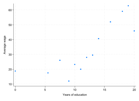
When working with micro-level data (i.e., unit is a firm, individual, household, etc.) you often need to aggregate the data to a lower level (e.g., region, group category). In Stata, this can be done using the collapse command. In R, you can use group_by() function within dplyr. This leads to an irreversible change in the structure of the dataset: you can aggregate data, but not disaggregate it. For this reason, it is a good idea to retain a version of the disaggregated data. In R, this is relatively straight forward because you can assign the aggregated file to a new dataframe. In Stata, you cannot have two datasets open at once. The solution therefore is to preserve a version of the disaggregated data and restore it once you are done with the aggregated file.

Note, preserve and restore must be run together. The command uses temporary files, so if you just run preserve and then later try to restore, the temporary file will no longer exist and you will need to re-open the disaggregated file and reproduce all other changes you made to the dataset.

For parts of the domain (i.e. years of education) the relationship does appear to be linear. This is for years of education from 10-19. Average wages decline beyond 19 and are flat (although noisy) below 10. This may be a sign that level of education matters above a minimum threshold; e.g. completing high school.

The plot below shows the average log of wage for each year of education. Does the relationship appear to be linear in years of education?

preserve
collapse (mean) lnwage, by(edu)
scatter lnwage edu, ytitle(Average (log of) wage) xtitle(Years of education)
restore

(Note: Below code run with echo to enable preserve/restore functionality.)

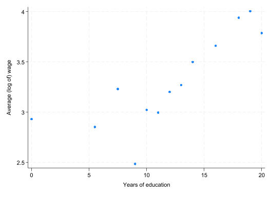
A similar pattern exists: linear within the domain 10-19 years of education. The log transformation is monotonic, but has a disproportionate impact on larger numbers (e.g. outliers). This may suggest that there are few outliers in the data.

Below is an estimate of the Mincer equation using the same sub-sample:

reg lnwage edu exp expsq


      Source |       SS           df       MS      Number of obs   =       300
-------------+----------------------------------   F(3, 296)       =     33.82
       Model |  26.8176018         3  8.93920059   Prob > F        =    0.0000
    Residual |  78.2323313       296  .264298417   R-squared       =    0.2553
-------------+----------------------------------   Adj R-squared   =    0.2477
       Total |  105.049933       299  .351337569   Root MSE        =     .5141

------------------------------------------------------------------------------
      lnwage | Coefficient  Std. err.      t    P>|t|     [95% conf. interval]
-------------+----------------------------------------------------------------
         edu |   .0998468   .0107859     9.26   0.000       .07862    .1210736
         exp |   .0208725   .0081481     2.56   0.011      .004837    .0369081
       expsq |  -.0002387    .000162    -1.47   0.142    -.0005575    .0000801
       _cons |   1.732044   .1753344     9.88   0.000     1.386984    2.077104
------------------------------------------------------------------------------

Interpret the coefficient on edu.

A 1 year increase in years of education increases predicted wages by approximately $\sim 10\%$, holding other factors constant. This coefficient is right on the edge of values for which it is appropriate to use the $\hat{\beta}\times 100$ approximation. The exact value is given by,

dis (exp(_b[edu])-1)*100

10.50016

which is slightly higher at 10.5%.

Ask a LLM to provide an estimate of the returns to an additional year of education from the literature. You must specify that the outcome is measured in log-of wages. What is the typical estimate? And do our estimates seem off?

A query, using Claude, cited a few key studies and meta-analyses. The conclusion was a range of 0.08-0.10; although it did specifiy a lower range of 0.06-0.07 for rich countries. This estimate is therefore slightly higher.

Can we reject the $H_0: \beta_1 <0.08$ at a $\alpha=0.01$ significance level? What if we chose $\alpha=0.05$ instead?

This test is designed to check whether or model estimates a return to education that is significantly higher than the using 0.08 value. It is a one-sided test, so we will reject if

\[ t\text{-stat} = \frac{\hat{\beta_1}-0.08}{se(\hat{\beta_1})}>t^{-1}_{300-4}(0.99) \]

Where $t^{-1}_{n-k-1}(\cdot)$ is the inverse of the CDF, so $t^{-1}_{300-4}(0.99)$ is the $99^{th}$ percentile of a $t$-distribution with 296 degrees of freedom.

dis (_b[edu]-0.08)/_se[edu]
dis invt(e(df_r),0.99)
dis invt(e(df_r),0.95)

1.8400626
2.3390116
1.6500177

We fail to reject this null hypothesis at 1% significance level. We would reject at a 5% level.

Test the hypothesis that $H_0:\beta_2=0$ at a $\alpha=0.05$ significance level.

This is a two-sided test. We will reject if,

\[ |t\text{-stat}| = \Bigg|\frac{\hat{\beta_2}}{se(\hat{\beta_2})}\Bigg|>t^{-1}_{300-4}(0.975) \]

dis _b[exp]/_se[exp]
dis invt(e(df_r),0.975)

2.56165
1.9680107

We reject this null hypothesis.

Test the hypothesis that $H_0:\beta_3\geq0$ at a $\alpha=0.05$ significance level.

This is a one-sided test. We will reject if,

\[ t\text{-stat} = \frac{\hat{\beta_3}}{se(\hat{\beta_3})}<t^{-1}_{300-4}(0.05) \]

dis _b[expsq]/_se[expsq]
dis invt(e(df_r),0.05)

-1.4736091
-1.6500177

We fail to reject this null hypothesis.

Ignoring statistical significance, do the estimates suggest a concave or convex relationship with respect to years of experience?

Since our estimate of $\hat{\beta}_3<0$, the data suggests that the relationship is concave. Wages are increasing in experience, but at a decreasing rate.

If we take these estimates seriously, after how many years of experience do we expected wages to decline? Do wages decrease while workers are still working?

For a quadratic function – $y = ax^2 + bx + c$ – the turning point is given by $-b/2a$

dis -_b[exp]/(2*_b[expsq])

43.719251

Wages reach their peak around 44 years of experience. This is close to retirement for most workers, so it suggests that wages continue to rise throughout a worker’s career.

Application 2: Explaining capital structures

The following model was inspired by Frank and Goyal (2009) Capital Structure Decisions: Which Factors Are Reliably Important?. The authors use a database of publicly-traded (US-listed) firms, from 1950-2003. They have a rich dataset of firm-level and macro-economic variables. In this example, we do not have that. Instead, we have data from the most recent SEC filings for 2026-Q2. Using this smaller cross-sectional dataset, we can estimate the model:

\[ leverage_i = \beta_0 + \beta_1 size_i + \beta_2 profitability_i + \beta_3 tangibility_i + u_i \]

where,

leverage: total liabilities divided by total assets
size: log of total assets
profitability: operating income divided by total assets
tangibility: physical assets (e.g., property and equipment) divided by total assets

The sample has been restricted to firms with assets of at least $1 million and a tangibility score within $[0,1]$.

sum leverage size profitability tangibility


    Variable |        Obs        Mean    Std. dev.       Min        Max
-------------+---------------------------------------------------------
    leverage |        271    1.311067    2.914094          0   22.16866
        size |        274     18.3593    2.601397   14.00696   26.29069
profitabil~y |        271    -.673556    2.286625  -29.20916   1.338037
 tangibility |        274    .1079863    .1624912          0   .9984815

reg leverage size profitability tangibility


      Source |       SS           df       MS      Number of obs   =       268
-------------+----------------------------------   F(3, 264)       =     29.28
       Model |    572.0114         3  190.670467   Prob > F        =    0.0000
    Residual |  1719.38448       264  6.51282001   R-squared       =    0.2496
-------------+----------------------------------   Adj R-squared   =    0.2411
       Total |  2291.39588       267  8.58200705   Root MSE        =     2.552

------------------------------------------------------------------------------
    leverage | Coefficient  Std. err.      t    P>|t|     [95% conf. interval]
-------------+----------------------------------------------------------------
        size |  -.2137509   .0642591    -3.33   0.001    -.3402764   -.0872253
profitabil~y |  -.5102825   .0724029    -7.05   0.000    -.6528431   -.3677218
 tangibility |    .868687   .9541517     0.91   0.363    -1.010029    2.747403
       _cons |   4.792315   1.208169     3.97   0.000     2.413441    7.171188
------------------------------------------------------------------------------

Interpret the $\mathbf{R}^2$ measure. Is this a high or low value?

The $\mathbf{R}^2=0.2496$. This tells us that 25% of the variation in the outcome is explained by the model (i.e. the regressors). It is difficult to say whether this is a high or low value, since different variables can be explained more/less by observable regressors. We can say that the value is no smaller than those found in the cited paper, which is somewhat surprising given that the authors include more regressors in their model (and $\mathbf{R}^2$ is weakly increasing in the number of regressors).

Interpret the _cons coefficient. Does this interpretation relate to a real firm?

Assuming that the error term has conditional mean zero, we can interpret the intercept as $E[y_i|\mathbf{x}_i=0]$. In this setting, this corresponds to the leverage of a firm with

size$=0\Rightarrow$ total assets of 1.
profitability$=0\Rightarrow$ zero profits
tangibility $=0\Rightarrow$ zero tengible assets

There is unlikely to be a firm of this nature in the SEC filings. Some firms may have zero profits, but SEC firms are unlikely to have total assets of $1.

Interpret each of the slope coefficients. For size, consider a 10% increase in assets. For profitability and tangibility, the regressor is a ratio. Consider the impact of an increase in the ratio of $\Delta x = 0.01$ (or 1%).

size: holding other factors fixed, a 10% increase in assets increases predicted leverage by

dis _b[size]*ln(1.1)

-.02037263

A reduction of 0.02 in leverage, or in 2% in liabilities as a share of assets.

profitability: holding other factors fixed, a 1% increase in profitability reduced predicted leverage (liabilities/assets) by 0.51%.
tangibility: holding other factors fixed, a 1% increase in tangibility increases predicted leverafe by 0.87%. However, this coefficient is not significantly different from 0.

These results are very different to those of Frank and Goyal (2009). For example, in their Table V the coefficient estimate for tangibility is $0.092$. What are some of the factors that could explain our vastly different results.

Here are a few factors to consider:

Time: this is a more recent dataset covering a very different macroeconomic environment. For example, interests have been historically low since the 2008 financial crisis. The authors also pool many years of data.
Sample selection: the datasets have different sample selection rules, which may lead to a sample representing a very different subset of US firms.
Model: the authors use a model with many more regressors: firm characteristics and macroeconomic variables not observed in this dataset. The estimates reported here may be effected by the absence of these other regressors. [Note: this is something called omitted variable bias, which we will discuss in Week 8.]

References

Card, David. 2001. “Estimating the Return to Schooling: Progress on Some Persistent Econometric Problems.” Econometrica 69 (5): 1127–60.

Frank, Murray Z, and Vidhan K Goyal. 2009. “Capital Structure Decisions: Which Factors Are Reliably Important?” Financial Management 38 (1): 1–37.

Lemieux, Thomas. 2006. “The ‘Mincer Equation’ Thirty Years After Schooling, Experience, and Earnings.” In Jacob Mincer a Pioneer of Modern Labor Economics, 127–45. Springer.

Mincer, Jacob. 1974. Schooling, Experience, and Earnings. New York: Columbia University Press.