Dynamic Documents with R and Quarto

Tayside Coding Club - 2 July 2026

Neil Lloyd

R Markdown

R users will be familiar with R markdown.

Markdown scripts (.Rmd) were designed specifically for R integration
Reverses the code-comment format of an .R script
- uncommented text is plain text and formatted based on standard markup syntax
- executable code is moved to a code-block.

For example,

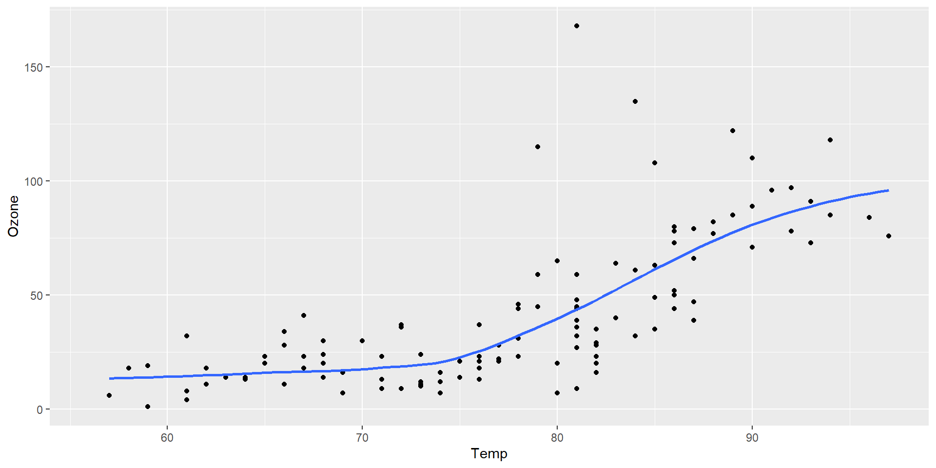
In the figure below you see a plot of temperature against ozone.  

```
library(ggplot2)
ggplot(airquality, aes(Temp, Ozone)) + 
  geom_point() + 
  geom_smooth(method = "loess", se = FALSE)
```

Quarto

Quarto is a more complete, open-source publishing system developed by Posit.¹

It works on the same basic principles as R Markdown but with more features and flexibility.

Why?

Accessibility: Creating digital resources solves a well known problem of screen readibility of PDF documents. Solve this problem by publishing simultaneously
- multiple formats: Word, PDF, HTML, etc.
Flexibility: write in markdown, publish as website, document, presentations, blog, dashboard, etc.
- more authentic and creative modes of assessment (in the age of AI)
- more modern, engaging material
Reproducibility: Incorporate reproducible code directly into your documents.
- along with data, tables, and figures
- using a range of languages: R, Python, Julia, even software like Stata
- sync changes through an online host (e.g. GitHub Pages)
Interactivity: Create “live” interactive documents that allow you to interact with data in real time.

Quarto markdown basics

Quarto markdown files (.qmd) work just like .Rmd files.

## New slide title

Add a list of

1. item 1
2. item 2

   a. sub-item 1
   
Add some maths: $\hat{\beta}$ is defined as

$$
  \hat{\beta} = (X'X)^{-1}X'Y
$$

:::{.callout-note title="Important"}
This is the most important equation in this module.
:::

They have a few nice features like callout blocks.

New slide title

Add a list of

item 1
item 2
1. sub-item 1

Add some maths: \(\hat{\beta}\) is defined as

\[ \hat{\beta} = (X'X)^{-1}X'Y \]

Important

This is the most important equation in this module.

Basics of R in Quarto

As with R markdown, you add R code inside a code block.

```{r}
library(ggplot2)
ggplot(airquality, aes(Temp, Ozone)) + 
  geom_point() + 
  geom_smooth(method = "loess", se = FALSE)
```

Basics of R in Quarto

This renders as follows:

Useful features for R users

#1 Echo the code

You can choose to echo the code by adding #| echo: true at the top of the code block.

library(ggplot2)
ggplot(airquality, aes(Temp, Ozone)) + 
  geom_point() + 
  geom_smooth(method = "loess", se = FALSE)

#2 Fold the code

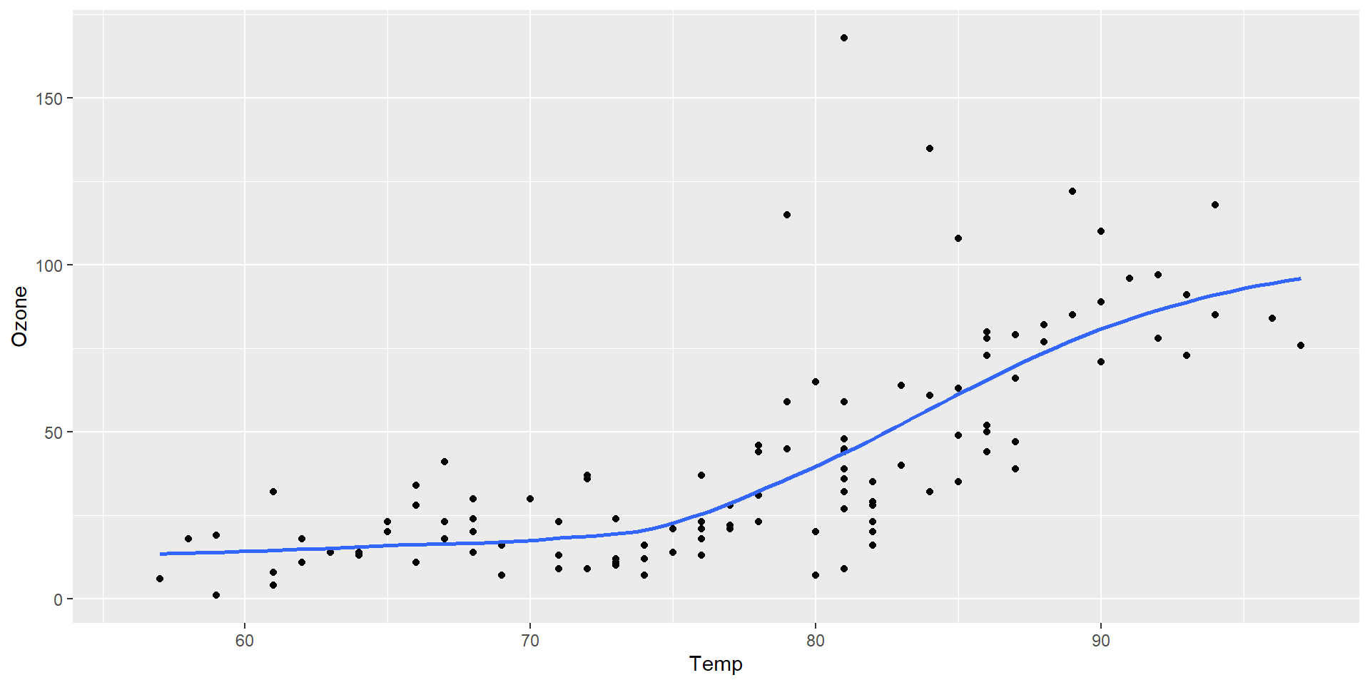
Adding the option #| code-fold: true will then fold the code block (when publishing as .html)

Code

library(ggplot2)
ggplot(airquality, aes(Temp, Ozone)) + 
  geom_point() + 
  geom_smooth(method = "loess", se = FALSE)

#3 Scrollable slides

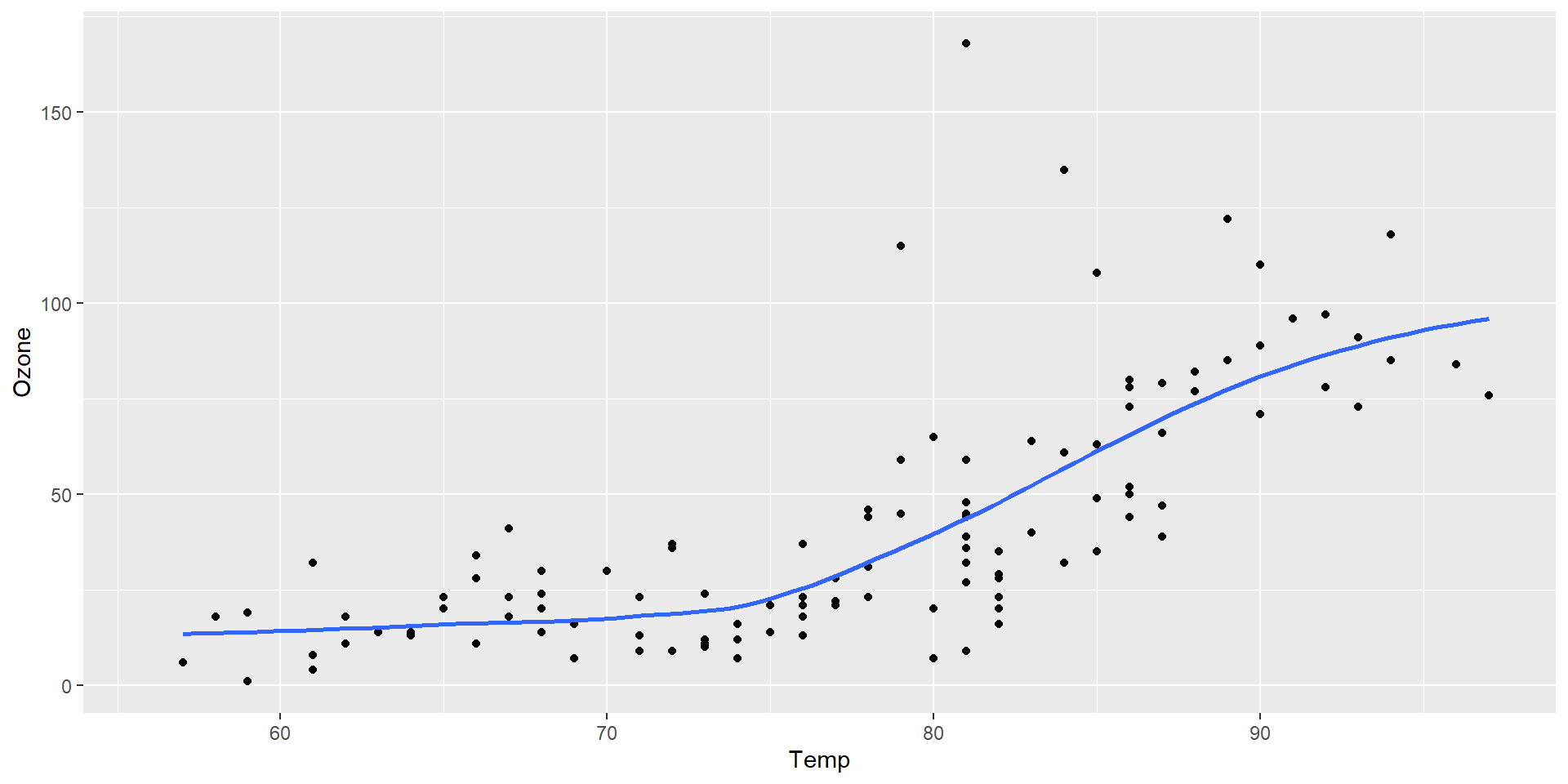
For revealjs slides, like these, the slide can be “scrollable” to ensure fit.

Code

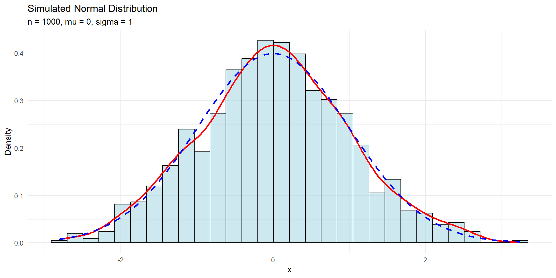
library(tibble)

set.seed(123)
n <- 1000
mu <- 0
sigma <- 1
df <- tibble(x = rnorm(n, mean = mu, sd = sigma))

gg <- ggplot(df, aes(x = x)) +
  geom_histogram(aes(y = ..density..), bins = 30, fill = "lightblue", color = "black", alpha = 0.6) +
  geom_density(color = "red", size = 1) +
  stat_function(fun = dnorm, args = list(mean = mu, sd = sigma), color = "blue", linetype = "dashed", size = 1) +
  labs(
    title = "Simulated Normal Distribution",
    subtitle = paste0("n = ", n, ", mu = ", mu, ", sigma = ", sigma),
    x = "x",
    y = "Density"
  ) +
  theme_minimal()
gg

#4 Tabs to split material

Alternatively, use tabs to display different components:

Code
Data
Plot

library(tibble)

set.seed(123)
n <- 1000
mu <- 0
sigma <- 1
df <- tibble(x = rnorm(n, mean = mu, sd = sigma))

gg <- ggplot(df, aes(x = x)) +
  geom_histogram(aes(y = ..density..), bins = 30, fill = "lightblue", color = "black", alpha = 0.6) +
  geom_density(color = "red", size = 1) +
  stat_function(fun = dnorm, args = list(mean = mu, sd = sigma), color = "blue", linetype = "dashed", size = 1) +
  labs(
    title = "Simulated Normal Distribution",
    subtitle = paste0("n = ", n, ", mu = ", mu, ", sigma = ", sigma),
    x = "x",
    y = "Density"
  ) +
  theme_minimal()

If you want to get fancy

Interactive material

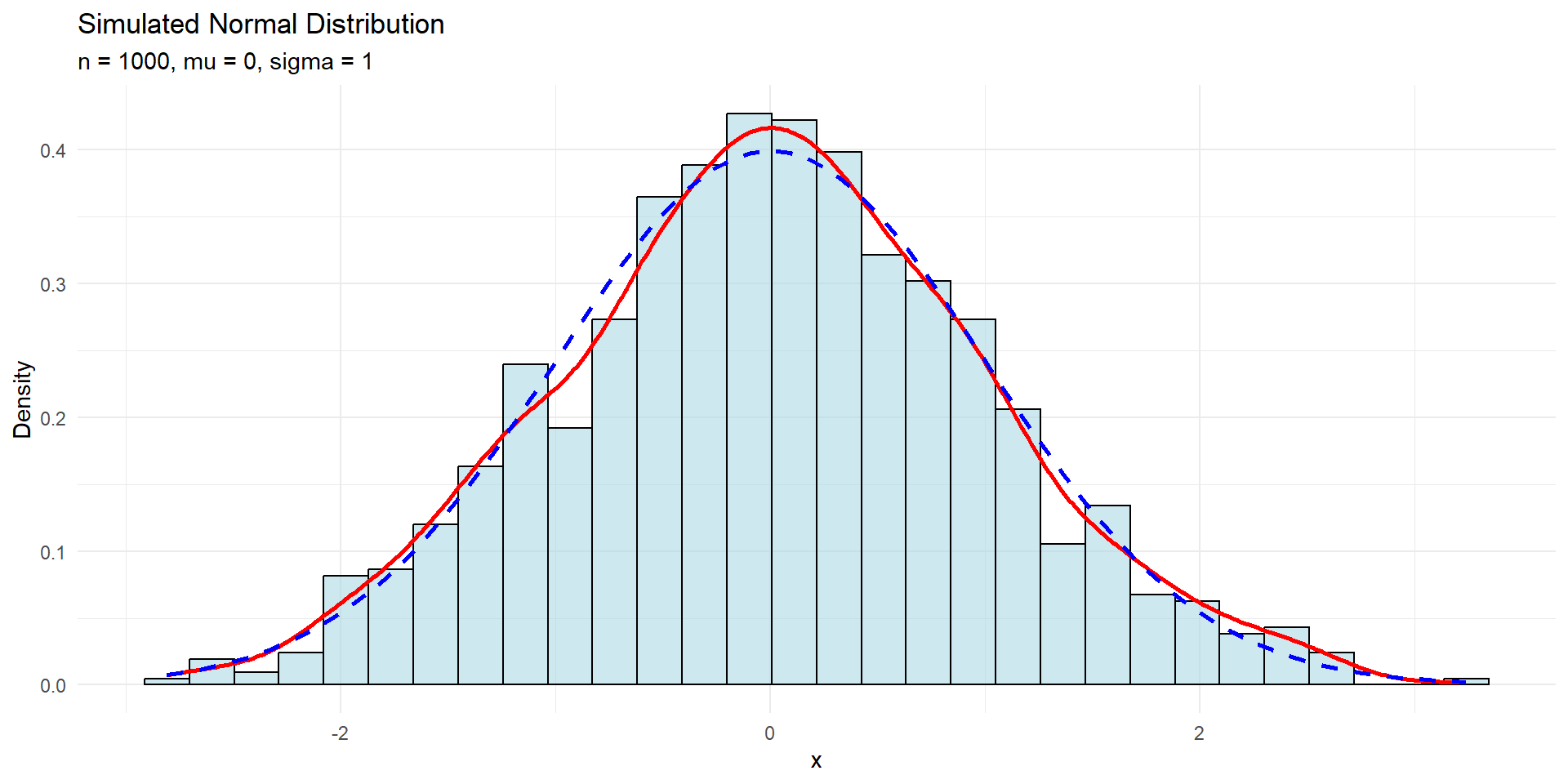
You can use Observable JS (within Quarto) to create interactive material.¹ Here is a simulation of the OLS estimator for different sample sizes.

\[ \begin{aligned} &Y_i = \beta_0 + \beta_1 X_i + \epsilon_i \\ \text{where}\;& \beta_0=2,\; \beta_1=1.5,\; X_i\sim U(0,10),\; \text{ and }\; \epsilon_i \sim N(0,3^2) \end{aligned} \]

viewof sample_size = Inputs.range(
  [10, 1000],
  {value: 500, step: 10, label: "Sample size"}
)

full_data = transpose(sim_data)
sample = full_data.slice(0, sample_size)

ols_result = {
  const n = sample.length;
  const x = sample.map(d => d.x);
  const y = sample.map(d => d.y);
  const xMean = d3.mean(x);
  const yMean = d3.mean(y);

  const num = d3.sum(x.map((xi, i) => (xi - xMean) * (y[i] - yMean)));
  const den = d3.sum(x.map(xi => (xi - xMean) ** 2));
  const slope = num / den;
  const intercept = yMean - slope * xMean;

  const residuals = x.map((xi, i) => y[i] - (intercept + slope * xi));
  const rss = d3.sum(residuals.map(r => r ** 2));
  const sigma2 = rss / (n - 2);
  const seSlope = Math.sqrt(sigma2 / den);
  const seIntercept = Math.sqrt(sigma2 * (1 / n + (xMean ** 2) / den));
  
  return { slope, seSlope, intercept, seIntercept, n };
}

html`<table>
  <thead>
    <tr><th>Parameter</th><th>Estimate</th><th>Std. Error</th></tr>
  </thead>
  <tbody>
    <tr><td>Constant (β₀)</td><td>${ols_result.intercept.toFixed(3)}</td><td>${ols_result.seIntercept.toFixed(3)}</td></tr>
    <tr><td>Slope (β₁)</td><td>${ols_result.slope.toFixed(3)}</td><td>${ols_result.seSlope.toFixed(3)}</td></tr>
  </tbody>
</table>`

More advanced versions require the use of a server.

Considerations

Here are a few things you will need to consider:

When publishing PDFs, troubleshooting and parcing settings to LaTeX can be a tricky!
Formatting html documents require the use of a CSS/SCSS style sheets.
- AI can help with this.
Markdown is an intentionally simple (easy-to-learn) language, but it is not as featureful as LaTeX.
- My least favourite feature is footnotes! 😔
Coding within a markdown file requires the use of code blocks.
- Not necessarily how you work (or want your students to engage with code).
- You can probably write a script to strip the code and create a .R script for your students to run.
You can create multi-lingual documents (R, Python, even Stata).
- There are some limitations and solutions. See my discussion here.

Questions

neil.lloyd@st-andrews.ac.uk / https://neil-lloyd.github.io/digital-resources/